Inside Retail Operations: A Case Study on Sales, Inventory, and Vendors
Table of Contents
1. INTRODUCTION
What does it take to run a successful liquor business? It’s not just about stocking popular products – it’s about understanding what sells, how fast it moves, and which vendors help or hurt your bottom line.
In this case study, we analyzes data from Bibitor, LLC – a fictional retail chain with 80+ locations and over $450M in annual sales, to uncover patterns patterns in vendor performance, inventory movement, and sales behavior, using real-world retail concepts.
🧾 About the Dataset
The dataset, obtained from the HUB of Analytics Education, simulates operational data from a large-scale liquor retailer based in Lincoln, USA, for the month of December 2016. It consists of six key data tables that collectively represent purchasing, inventory, sales, and vendor transactions.
- Inventory
BegInvDec: Inventory at the start of December 2016.EndInvDec: Inventory remaining at the end of December 2016.
- Purchases
PurchasesDec: What Bibitor bought from vendors (quantities, total cost, vendor info).PricingPurchasesDec: Reference prices Bibitor expects from suppliers.
- Vendor Invoices
VendorInvoicesDec: The bills Bibitor received from their suppliers (vendors).
- Sales
SalesDec: Item-level sales data including price, quantity, and total revenue.
When combined, these tables allow us to track products from purchase to sale, understand vendor relationships, and monitor financial flows, which are all crucial for optimizing retail operations.
🔑 Key Business Questions
- Which vendors offer the highest value?
- Are we overstocking or underutilizing inventory?
- How do purchase prices compare to actual sales?
- What’s the average time it takes to sell received stock?
- Are our product costs accurately reflecting ongoing purchase fluctuations?
🧩 Data Model
Before diving into the code, we first need to understand how all the different pieces of data connect. An Entity-Relationship Diagram (ERD) visually represents these connections, providing the logical framework for accurate and efficient analysis. This ensures our data joins are correct and our derived insights are reliable.
The ERD below guided our analysis, showing the relationships between Bibitor’s core transactional and master data tables:
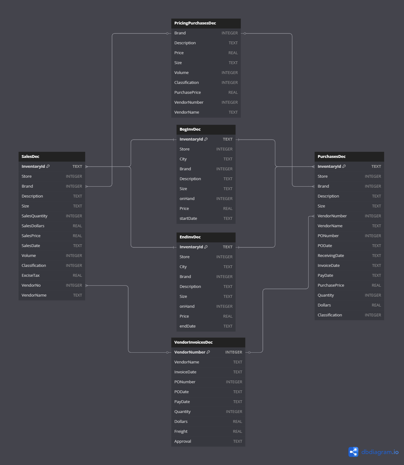
As shown, tables like PurchasesDec and VendorInvoicesDec are linked by a shared key like VendorNumber. This forms the core of Bibitor’s purchasing data. Table SalesDec then links via InventoryId to track items’ journeys from purchase to customer. This setup creates a smooth flow for tracing items and understanding all financial transactions across the business.
2. ANALYSIS WITH SQL
SQL was our main tool for extracting, transforming, and initially analyzing Bibitor’s extensive datasets. Its strong querying abilities let us take a structured and detailed approach to answer important business questions.
All SQL scripts used in this analysis are available in the following GitHub repository:
2.1. Initial Data Health Check
📜 SQL Script: 01. Initial Analysis.sql
We began our analysis by thoroughly ensuring data integrity. This involved systematic checks for missing values, zero balances in key financial data, and inconsistencies, all of which could impact the reliability of our findings.
🔑 Key Objectives:
- Identify missing or zero values in sales, purchases, or pricing data.
- Assess the completeness and overall cleanliness of the entire dataset.
- Verify that calculated fields (e.g.,
PurchasePrice * Quantity) accurately match recorded totals. - Ensure vendor information is consistent across all related tables.
🔍 A glimpse into the Code:
a. Missing or Zero values
📦 Purchases:
SELECT * FROM PurchasesDec WHERE Dollars <= 0 OR Dollars IS NULL;
Sample Output:
| InventoryId | Store | Brand | … | VendorNumber | VendorName | PONumber | PODate | ReceivingDate | InvoiceDate | PayDate | PurchasePrice | Quantity | Dollars |
|---|---|---|---|---|---|---|---|---|---|---|---|---|---|
| 59_CLAETHORPES_2166 | 59 | 2166 | … | 2561 | EDRINGTON AMERICAS | 11462 | 2016-08-02 | 2016-08-10 | 2016-08-22 | 2016-10-01 | 0 | 12 | 0 |
| 38_GOULCREST_2166 | 38 | 2166 | … | 2561 | EDRINGTON AMERICAS | 11462 | 2016-08-02 | 2016-08-11 | 2016-08-22 | 2016-10-01 | 0 | 12 | 0 |
| 34_PITMERDEN_2166 | 34 | 2166 | … | 2561 | EDRINGTON AMERICAS | 11462 | 2016-08-02 | 2016-08-09 | 2016-08-22 | 2016-10-01 | 0 | 12 | 0 |
| 44_PORTHCRAWL_2166 | 44 | 2166 | … | 2561 | EDRINGTON AMERICAS | 11462 | 2016-08-02 | 2016-08-08 | 2016-08-22 | 2016-10-01 | 0 | 12 | 0 |
| 56_BEGGAR’S HOLE_2166 | 56 | 2166 | … | 2561 | EDRINGTON AMERICAS | 11462 | 2016-08-02 | 2016-08-09 | 2016-08-22 | 2016-10-01 | 0 | 12 | 0 |
Our query returned 153 records where the Dollars value is zero or null. Given that Dollars is calculated from PurchasePrice * Quantity, a zero value here strongly suggests these items had a zero purchase price. Possible explanations include:
- Promotional or Free Goods: These items might have been given away as part of a marketing campaign, a promotion, or bundled with other purchases.
- Samples: They could also be products recorded as samples for in-store use or customer trials.
- Data Entry Errors: Mistakes made during data input.
📦 Sales:
SELECT * FROM SalesDec WHERE SalesDollars <= 0 OR SalesDollars IS NULL;
Sample Output:
| InventoryId | Store | Brand | … | SalesQuantity | SalesDollars | SalesPrice | SalesDate | Classification | ExciseTax | VendorNo | VendorName |
|---|---|---|---|---|---|---|---|---|---|---|---|
| 38_GOULCREST_25340 | 38 | 25340 | … | 3 | 0 | 0 | 2016-02-13 | 2 | 0.34 | 4425 | MARTIGNETTI COMPANIES |
| 66_EANVERNESS_25340 | 66 | 25340 | … | 3 | 0 | 0 | 2016-02-12 | 2 | 0.34 | 4425 | MARTIGNETTI COMPANIES |
| 66_EANVERNESS_25340 | 66 | 25340 | … | 1 | 0 | 0 | 2016-02-16 | 2 | 0.11 | 4425 | MARTIGNETTI COMPANIES |
| 67_EANVERNESS_25340 | 67 | 25340 | … | 12 | 0 | 0 | 2016-02-07 | 2 | 1.35 | 4425 | MARTIGNETTI COMPANIES |
| 73_DONCASTER_25340 | 73 | 25340 | … | 1 | 0 | 0 | 2016-02-15 | 2 | 0.11 | 4425 | MARTIGNETTI COMPANIES |
We found 55 sales records with zero or missing sales amounts, meaning these transactions were recorded with a zero sales price.
➡️ Next steps:
To figure out if these zero-value entries are valid, we need to take a few more steps:
- Talk to our business teams to confirm if these types of transactions are expected in certain situations, like promotions.
- Analyzing patterns by product or vendor to identify systematic issues.
- Reviewing pricing and promotional strategies. This might help explain why some transactions show zero dollars.
- Investigating potential data entry or system integration errors.
b. Percentage of Zero or Null in the dataset
The percentage of zero or null monetary values in the datasets was calculated to evaluate overall data quality:
SELECT
    CAST(SUM(CASE WHEN Dollars <= 0 OR Dollars IS NULL THEN 1 ELSE 0 END) AS REAL) * 100 / COUNT(*) AS ZeroPurchases
FROM PurchasesDec;
Output: 0.0064
SELECT
    CAST(SUM(CASE WHEN SalesDollars <= 0 OR SalesDollars IS NULL THEN 1 ELSE 0 END) AS REAL) * 100 / COUNT(*) AS ZeroSales
FROM SalesDec;
Output: 0.0004
➡️ These very low percentages show that our financial data is exceptionally clean regarding zero or missing monetary values. This is a significant advantage for the quality of any future analysis.
c. Dataset Summaries
This section provides a foundational overview of our datasets’ key characteristics.
📦 Purchases:
The PurchasesDec table contains 2.37 million rows, representing purchases from 128 distinct vendors across 5,543 unique purchase orders. Here are the key statistics for monetary values and quantities:
| Metric | Quantity (units) | Dollars |
|---|---|---|
| Total | 33,584,377 | $321,900,765.50 |
| Average | 14.16 | $135.68 |
| Minimum | 1 | $0.00 |
| Maximum | 3,816 | $50,175.70 |
The purchase data spans:
| Date Type | Start Date | End Date |
|---|---|---|
| PO Date | 2015-12-20 | 2016-12-23 |
| Receiving Date | 2016-01-01 | 2016-12-31 |
| Invoice Date | 2016-01-04 | 2017-01-10 |
| Pay Date | 2016-02-04 | 2017-02-19 |
📦 Sales:
The SalesDec table shows a total sales volume of $452,062,952 with an average sale amount of $35.25. Individual sales range from $0 to $26,061.14.
📦 Vendors:
The VendorInvoicesDec table shares similar date ranges with PurchasesDec for PO, Invoice, and Pay dates.
| Metric | Quantity (units) | Dollars | Freight |
|---|---|---|---|
| Total | 33,584,377 | $321,900,765.50 | $1,640,474.69 |
| Average | 6,058.88 | $58,073.38 | $295.95 |
| Minimum | 1 | $4.14 | $0.02 |
| Maximum | 141,660 | $1,660,435.88 | $8,468.22 |
2.2. Vendor Performance Analysis
📜 SQL Script: 02. Vendor Analysis.sql
The next phase of our analysis focused on Bibitor’s key relationships with its vendors and suppliers. Our goal was to get a complete, 360-degree view of vendor performance. This meant identifying our top suppliers, evaluating how efficient their shipping costs were, and measuring the profit each vendor’s products brought in.
🔑 Key Objectives:
- Top Vendor identification: Which vendors rank highest by total purchase spend, sales generated, and quantity of products we purchased from them?
- Item-level sales performance: What are the best-selling products supplied by each vendor?
- Freight cost insights: How significant are shipping costs compared to the purchase value for each vendor?
- Profitability assessment: What gross margin is generated from products supplied by each vendor, revealing their true profit contribution?
- Temporal trends: How do purchase and sales volumes change over time, and how can this help us spot seasonality or growth patterns?
🔍 A glimpse into the Code:
The first step involved compiling a comprehensive list of unique vendors by combining purchase and invoice data, yielding a total of 128 distinct suppliers.
a. Top Vendors by Spend & Revenue:
Understanding where the most capital is invested and which vendors drive sales revenue is critical. The query below ranks suppliers based on total purchase expenditure:
-- Identifies top 5 suppliers by total spending (Dollars)
SELECT
    VendorNumber,
    VendorName,
    SUM(Dollars) AS TotalPurchaseDollars
FROM PurchasesDec
GROUP BY VendorNumber, VendorName
ORDER BY TotalPurchaseDollars DESC
LIMIT 5;
Output 1:
| VendorNumber | VendorName | TotalPurchaseDollars |
|---|---|---|
| 3960 | DIAGEO NORTH AMERICA INC | $50,959,796.85 |
| 4425 | MARTIGNETTI COMPANIES | $27,861,690.02 |
| 12546 | JIM BEAM BRANDS COMPANY | $24,203,151.05 |
| 17035 | PERNOD RICARD USA | $24,124,091.56 |
| 480 | BACARDI USA INC | $17,624,378.72 |
Similarly, the analysis also identified the top suppliers by the total revenue generated from their products:
-- Identifies top 5 suppliers by total revenue (SalesDollars)
SELECT
  VendorNo AS VendorNumber,
  VendorName,
  SUM(SalesDollars) AS TotalSalesDollars
FROM SalesDec
GROUP BY VendorNo, VendorName
ORDER BY TotalSalesDollars DESC
LIMIT 5;
Output 2:
| VendorNumber | VendorName | TotalSalesDollars |
|---|---|---|
| 3960 | DIAGEO NORTH AMERICA INC | $68,742,416.99 |
| 4425 | MARTIGNETTI COMPANIES | $41,047,306.30 |
| 17035 | PERNOD RICARD USA | $32,281,247.95 |
| 12546 | JIM BEAM BRANDS COMPANY | $31,906,320.54 |
| 480 | BACARDI USA INC | $25,014,556.89 |
Both results consistently showed the same top performers in both purchase spend and sales revenue. Specifically, DIAGEO NORTH AMERICA INC stood out as the largest supplier, indicating strong alignment between what Bibitor buys and what their customers want.
b. Top-Selling Products by Vendor:
To gain a closer look at individual products, we identified each vendor’s top-selling item by aggregating sales quantities and revenues for all products they supplied, then ranking them accordingly.
Sample Output:
| VendorNumber | InventoryId | TotalSold | TotalSales |
|---|---|---|---|
| 2 | 76_DONCASTER_90609 | 23 | $574.77 |
| 60 | 73_DONCASTER_3979 | 9282 | $158,247.18 |
| 105 | 76_DONCASTER_8412 | 450 | $22,495.50 |
| 200 | 12_LEESIDE_20789 | 76 | $1,367.24 |
| 287 | 65_LUTON_24922 | 20 | $281.80 |
This detailed data will help us with targeted inventory management, planning promotions, and refining the product mix for every vendor.
c. Freight Cost Efficiency:
Shipping costs can really impact how much a product ultimately costs. So, instead of just looking at the total freight expenses, we evaluated freight as a percentage of the total purchase cost to identify inefficiencies:
-- Calculates and ranks vendors by freight cost as a percentage of their total purchase cost
SELECT
    VendorNumber,
    VendorName,
    SUM(Dollars) AS TotalPurchase,
    SUM(Freight) AS TotalFreight,
    ROUND(SUM(Freight) * 100.0 / NULLIF(SUM(Dollars), 0), 2) AS FreightPercent
FROM VendorInvoicesDec
GROUP BY VendorNumber, VendorName
ORDER BY FreightPercent DESC
LIMIT 5;
Output:
| VendorNumber | VendorName | TotalPurchase | TotalFreight | FreightPercent |
|---|---|---|---|---|
| 9625 | WESTERN SPIRITS BEVERAGE CO | $361,249.21 | $1,933.19 | 0.54% |
| 28776 | TALL SHIP DISTILLERY LLC | $48,445.58 | $259.90 | 0.54% |
| 3951 | HIGHLAND WINE MERCHANTS LLC | $5,500.32 | $29.43 | 0.54% |
| 1590 | DIAGEO CHATEAU ESTATE WINES | $1,365,472.83 | $7,259.75 | 0.53% |
| 9744 | FREDERICK WILDMAN & SONS | $759,449.24 | $3,999.93 | 0.53% |
The result showed that vendors with the highest freight costs as a percentage of total purchase cost weren’t always the ones with the highest total shipping expenses. This suggests that smaller or more specialized vendors may have less efficient shipping processes, causing freight to make up a larger portion of their product’s overall cost.
d. Profitability via Gross Margin:
One of the most important financial measures for evaluating vendors is Gross Margin. This metric compares how much revenue (sales) a vendor generates against the cost of the products purchased from them. It helps Bibitor understand which suppliers are not just efficient but also contribute the most to the company’s overall profitability — showing real dollars earned, not just percentages.
The SQL query below calculates both Gross Profit (the dollar amount earned after costs) and Gross Margin Percentage (profit as a share of revenue) for each vendor. This helps Bibitor focus on the top-performing suppliers:
-- Calculates the Gross Margin (Profit) by comparing Total Cost (Purchases) to Total Revenue (Sales) for each vendor
WITH Purchases AS (
    SELECT VendorNumber, SUM(Dollars) AS TotalCost FROM PurchasesDec WHERE Dollars > 0 GROUP BY VendorNumber
),
Sales AS (
    SELECT VendorNo AS VendorNumber, SUM(SalesDollars) AS TotalRevenue FROM SalesDec GROUP BY VendorNo
)
SELECT
    s.VendorNumber,
    s.TotalRevenue,
    p.TotalCost,
    (s.TotalRevenue - p.TotalCost) AS GrossProfit,
    ROUND((s.TotalRevenue - p.TotalCost) * 100.0 / NULLIF(s.TotalRevenue, 0), 2) AS GrossMarginPercent
FROM Sales s
LEFT JOIN Purchases p ON s.VendorNumber = p.VendorNumber
ORDER BY GrossProfit DESC
LIMIT 5;
Output:
| VendorNumber | TotalRevenue | TotalCost | GrossProfit | GrossMarginPercent |
|---|---|---|---|---|
| 3960 | $68,742,416.99 | $50,959,796.85 | $17,782,620.14 | 25.87% |
| 4425 | $41,047,306.30 | $27,861,690.02 | $13,185,616.28 | 32.12% |
| 1392 | $24,469,172.93 | $15,573,917.90 | $8,895,255.03 | 36.35% |
| 17035 | $32,281,247.95 | $24,124,091.56 | $8,157,156.39 | 25.27% |
| 12546 | $31,906,320.54 | $24,203,151.05 | $7,703,169.49 | 24.14% |
For example, Vendor 3960 has a lower Gross Margin Percentage than Vendor 1392, but because it sells a much larger volume, it contributes the most profit overall.
By looking at both absolute profit (Gross Profit dollars) and efficiency (Gross Margin Percentage), this analysis gives Bibitor a balanced perspective to make smarter decisions when managing vendor relationships. They can prioritize suppliers who maximize profitability and strengthen their negotiation position.
2.3. Inventory Turnover Analysis
📜 SQL Script: 03. Inventory Turnover Analysis.sql
Efficient inventory management is crucial for any retail business, as it directly impacts cash flow and profits. For this analysis, we focused on how quickly products move from purchase to sale. This helps us identify items that remain on shelves too long, which can tie up money and occupy valuable storage space.
a. Calculating “Days to Sell”:
Our key metric here is “Days to Sell” — the number of days it takes for a product to go from arrival in the store to its first sale. To calculate this, we simply each product’s received date with its first sale date. The results are stored in a new table called InventorySaleLag for easy review.
Although the full SQL script is detailed, the core idea is simple: we combined purchase and sales data to find the time difference between arrival and sale for each product at every store.
b. Identifying Slow-Moving Inventory:
With the InventorySaleLag data ready, we ran a simple query to flag slow-moving items—products that took more than 60 days to sell after arriving. Identifying these items helps the business take action, such as applying discounts or adjusting stock levels, to free up cash and valuable storage space.
-- Selects inventory items that took longer than 60 days to sell from the calculated data
SELECT
    InventoryId, Store, VendorName, AvgPurchasePrice, AvgSalesPrice,
    TotalPurchased, TotalSold, FirstReceived, FirstSold, DaysToSell
FROM InventorySaleLag
WHERE DaysToSell > 60
ORDER BY DaysToSell DESC
LIMIT 5;
Sample Output:
| InventoryId | Store | VendorName | … | TotalSold | FirstReceived | FirstSold | DaysToSell |
|---|---|---|---|---|---|---|---|
| 29_AYLESBURY_42188 | 29 | MOET HENNESSY USA INC | … | 1 | 2016-01-02 | 2016-12-31 | 364 |
| 29_AYLESBURY_2767 | 29 | DIAGEO NORTH AMERICA INC | … | 1 | 2016-01-02 | 2016-12-29 | 362 |
| 29_AYLESBURY_8897 | 29 | MOET HENNESSY USA INC | … | 2 | 2016-01-08 | 2016-12-31 | 358 |
| 5_SUTTON_17967 | 5 | BANFI PRODUCTS CORP | … | 1 | 2016-01-02 | 2016-12-22 | 355 |
| 6_GOULCREST_4574 | 6 | REMY COINTREAU USA INC | … | 1 | 2016-01-04 | 2016-12-22 | 353 |
The result quickly highlighted specific products that stay in stock for unusually long times. Some even sit on shelves for almost a full year! Items that remain unsold for too long increase storage costs. They also risk becoming outdated or unsellable, and tie up funds that could be better used elsewhere. By identifying these slow-moving products, Bibitor can take specific actions such as adjusting future orders, launching special promotions, or changing prices to improve sales and free up resources.
2.4. Inventory Valuation: Moving Average Cost (MAC)
📜 SQL Script: 04. Inventory MovingAvgCost.sql
Understanding the true cost of inventory is just as important as knowing how fast it sells. Bibitor can estimate this using the Moving Average Cost (MAC) method. This approach continuously updates each item’s average cost whenever new stock is bought, giving us the most current inventory value.
The process combines data on current stock, new purchases, and sales. Then, it calculates an up-to-date average cost for every product.
Calculating MAC:
To determine the Moving Average Cost, we followed a few key steps:
- Tracked sales and purchases: We recorded sales as negative quantities (items leaving stock) and purchases as positive quantities (items coming in) to accurately reflect inventory changes.
- Combined all transactions: All inventory movements, both incoming and outgoing, were merged into a single dataset for analysis.
- Added Beginning Inventory: We added the inventory available at the start of the month to get a complete picture of stock availability.
- Calculated Moving Average: For each product at every store, we divided the total cost of inventory by the total quantity on hand. This gives us a dynamic average cost that adjusts with new purchases and sales.
- Compared with Ending values: Finally, we compared the calculated average cost with the recorded inventory value at the end of the period to ensure accuracy.
Our goal was to maintain a precise and current average cost for every product. This helps Bibitor make informed decisions regarding pricing, budgeting, and overall profitability.
-- Calculate Moving Average Cost (MAC)
SELECT
    InventoryId,
    Store,
    Brand,
    SUM(Quantity) AS Quantity,
    SUM(Price) AS TotalCost,
    (SUM(Price) / NULLIF(SUM(Quantity), 0)) AS MAC
FROM temp.BegInv_andTrans_proc
GROUP BY InventoryId, Store, Brand;
Sample Output:
| Inventory ID | Store | City | Brand | Description | Size | On Hand | Price ($) | End Date | MAC ($) | Difference ($) |
|---|---|---|---|---|---|---|---|---|---|---|
| 10_HORNSEY_1001 | 10 | HORNSEY | 1001 | Baileys 50mL 4 Pack | 50mL 4 Pk | 0 | 5.99 | 2016-12-31 | 0.5445 | 5.4455 |
| 10_HORNSEY_1003 | 10 | HORNSEY | 1003 | Crown Royal VAP Glass+Coaster | 750mL | 73 | 22.99 | 2016-12-31 | 3.1519 | 19.8381 |
| 10_HORNSEY_10058 | 10 | HORNSEY | 10058 | F Coppola Dmd Ivry Cab Svgn | 750mL | 24 | 14.99 | 2016-12-31 | 0.5915 | 14.3985 |
| 10_HORNSEY_10062 | 10 | HORNSEY | 10062 | B de Beauchene CDR Rouge | 750mL | 15 | 8.99 | 2016-12-31 | 0.8173 | 8.1727 |
| 10_HORNSEY_10164 | 10 | HORNSEY | 10164 | Andre Bourgogne Pnt Nr RSV | 750mL | 19 | 15.99 | 2016-12-31 | 1.4536 | 14.5364 |
3. DASHBOARD VISUALIZATIONS
3.1. Vendor Performance & Financial Overview
a. Understanding Business Flow
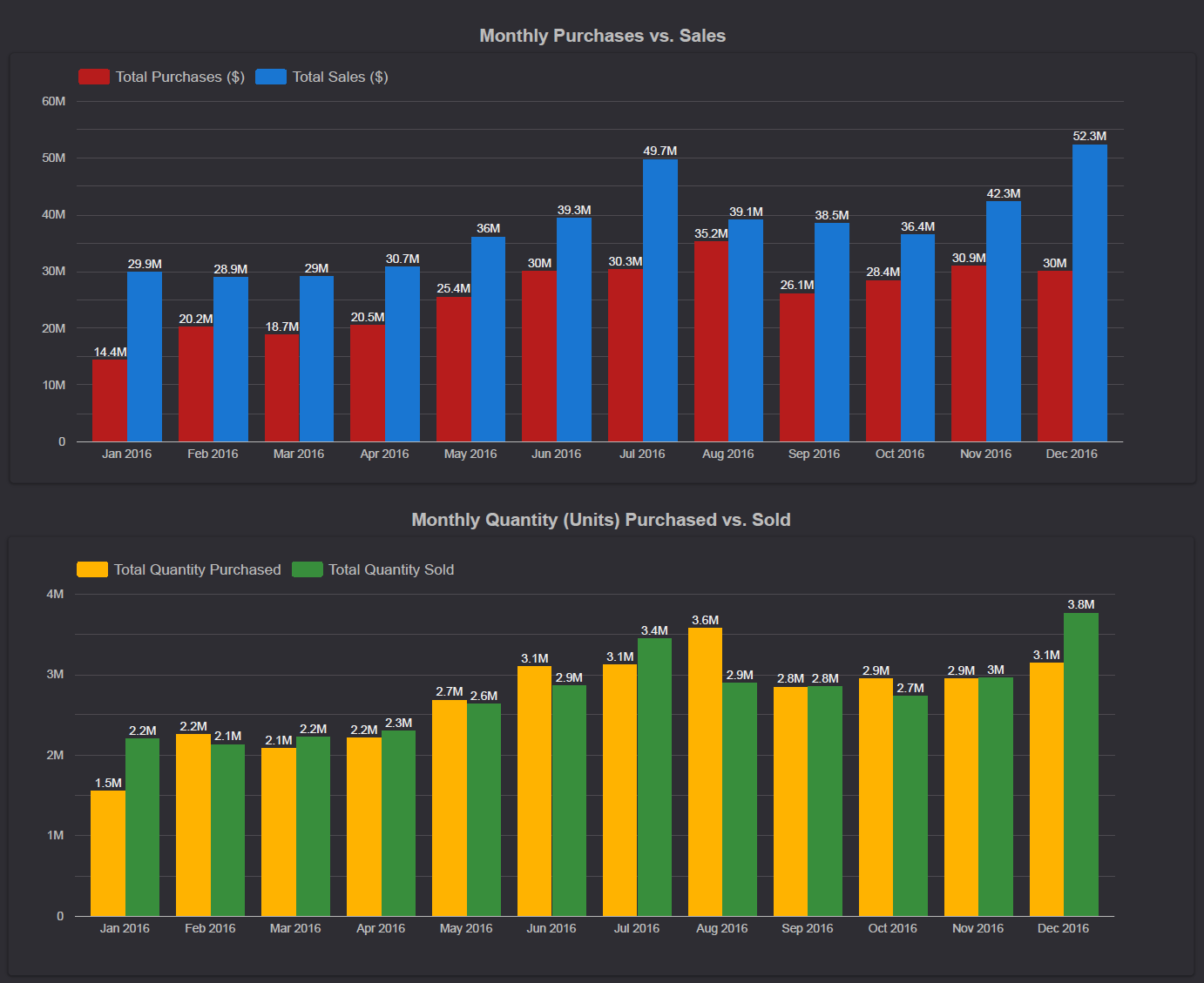
Monthly trends in purchases and sales reveal key patterns in Bibitor’s business flow. These insights support smarter inventory planning and financial forecasting:
- Purchases steadily increased through 2016, hitting their highest point in August, which likely means inventory was being built up.
- Sales showed sharper growth, especially in July and December. This points to strong seasonality, probably linked to summer and holiday demand.
Understanding these rhythms helps us ensure we stock the right products at the right times.
b. Visualizing Vendor Dominance
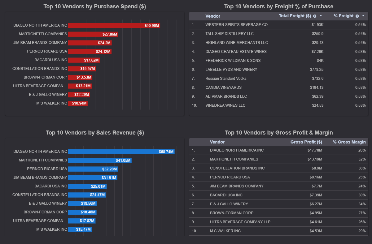
This section showcases top-performing vendors through key financial metrics: Purchase Spend, Sales Revenue, and Gross Profit/Margin. As noted earlier (Section 2.2), DIAGEO NORTH AMERICA INC consistently ranks highest, clearly standing out across all metrics.
The bar charts clearly rank vendor performance, making it easy to compare their impact on Bibitor’s profits. At the same time, the “Top 10 Vendor by Freight % of Purchase” table highlights shipping efficiency problems. It shows that some smaller vendors might have disproportionately high freight costs compared to the size of their orders.
c. Vendor Inventory Insights
A new dimension of analysis focuses on inventory allocation across vendors:
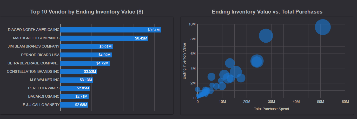
- Ending Inventory Value: The “Top 10 Vendor by Ending Inventory Value ($)” bar chart shows where most of Bibitor’s current stock value is concentrated. DIAGEO NORTH AMERICA INC again leads, followed by Martignetti Companies. This reflects not only their high purchase volumes but also a slower turnover of their products.
- Inventory vs. Purchases: The scatter plot “Ending Inventory Value vs. Total Purchases” shows that vendors who buy more also tend to hold more ending inventory. The large bubbles in the upper-right corner (e.g., DIAGEO NORTH AMERICA INC) indicate high capital investment and the need to monitor stock efficiency.
📝 Summary
This dashboard effectively transforms complex vendor data into actionable insights. By spotlighting our top vendors across purchases, sales, profitability, and inventory, Bibitor can better prioritize key relationships, assess capital allocation, and refine stock strategies. These insights are vital for driving sustainable growth.
3.2. Inventory Efficiency & Product-Level Insights
This dashboard is designed to support strategic vendor relationships by offering clear insights into Bibitor’s inventory health and product flow. It offers clear insights into how quickly products move, identifies bottlenecks, and highlights both strong performers and areas needing immediate attention.
a. Highlighting Product Successes
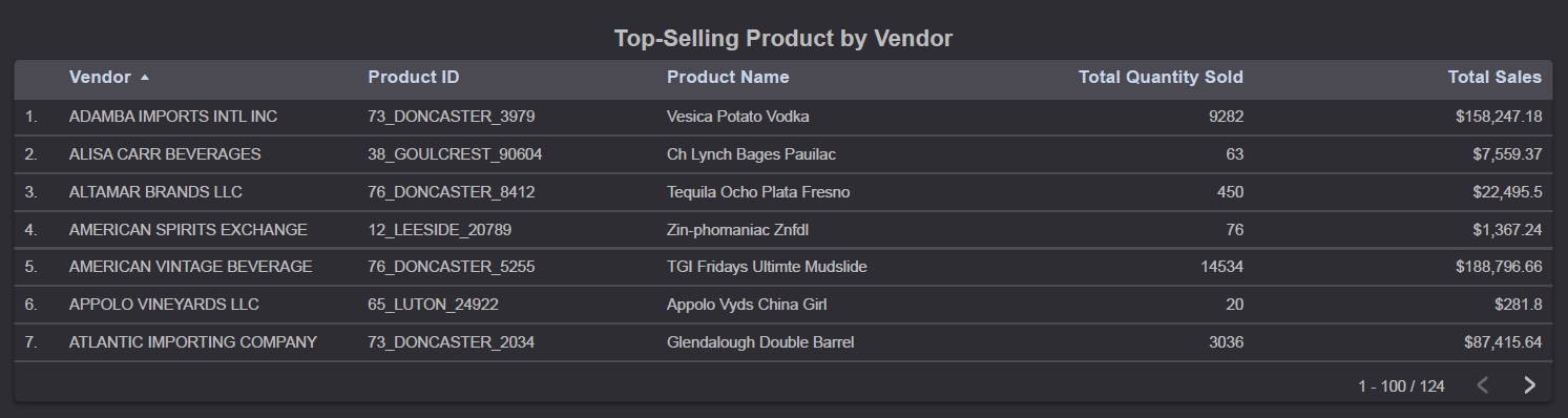
The “Top-Selling Product by Vendor” table clearly displays each vendor’s best-selling item based on both quantity sold and total sales. This helps us identify specific high-performing products to keep in stock and focus on in marketing. It also highlights the overall vendor performance by showing which specific product drives the most success for each vendor within Bibitor.
b. Inventory Velocity
This section visualizes how quickly products sell after arriving in inventory, based on the “Days to Sell” metric introduced in Section 2.3.
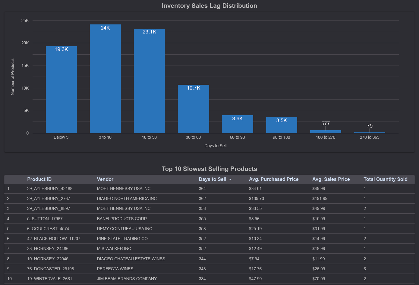
- Overall Sales Lag Distribution: The “Inventory Sales Lag Distribution” chart gives a clear overview of inventory turnover. Most of Bibitor’s products sell within a short time, usually under 30 days. However, it also highlights a “long tail” — a smaller, but significant, number of products that stay in inventory for a long time, sometimes 90 days or more. These items tie up our cash and storage space.
- Identifying Slow Movers: The accompanying table lists the ten products with the longest sales lag, including product and vendor details. These are ideal candidates for promotions, pricing changes, or a full stock review.
c. Performance Drivers: By Vendor and By Store
 To pinpoint where slow-moving inventory originates:
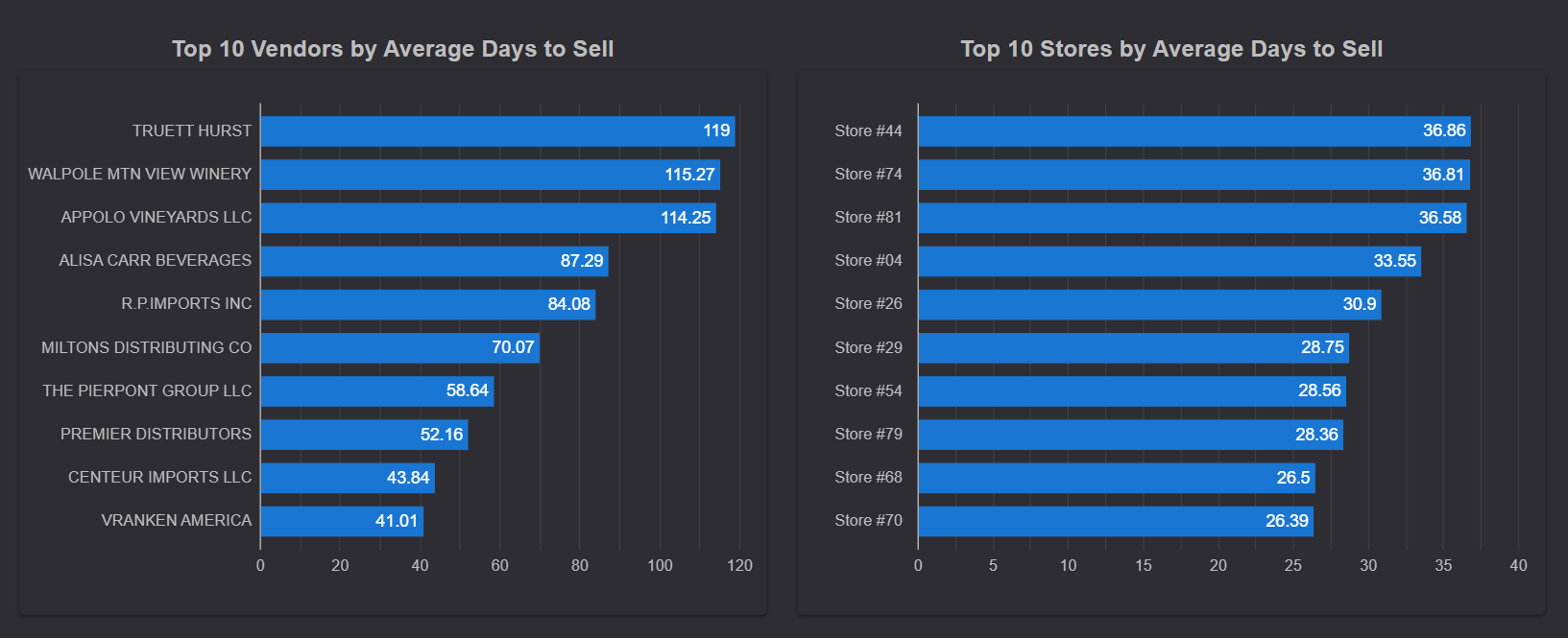
- Vendor Performance: The “Top 10 Vendors by Average Days to Sell” chart clearly shows which suppliers are linked to slower-moving inventory. For instance, TRUETTI HURST and WALPOLE MTN VIEW WINERY stand out with significantly higher average days to sell (119 and 115 days, respectively). This insight can lead to discussions about their product mix, alignment with customer demand, or purchasing volumes.
- Store Performance: The “Top 10 Stores by Average Days to Sell” chart highlights locations where inventory tends to sit longer. Stores #44 and #74 have higher average days to sell (36–37 days), indicating potential local demand issues, merchandising problems, or inventory management inefficiencies.
d. Inventory Cost & Valuation
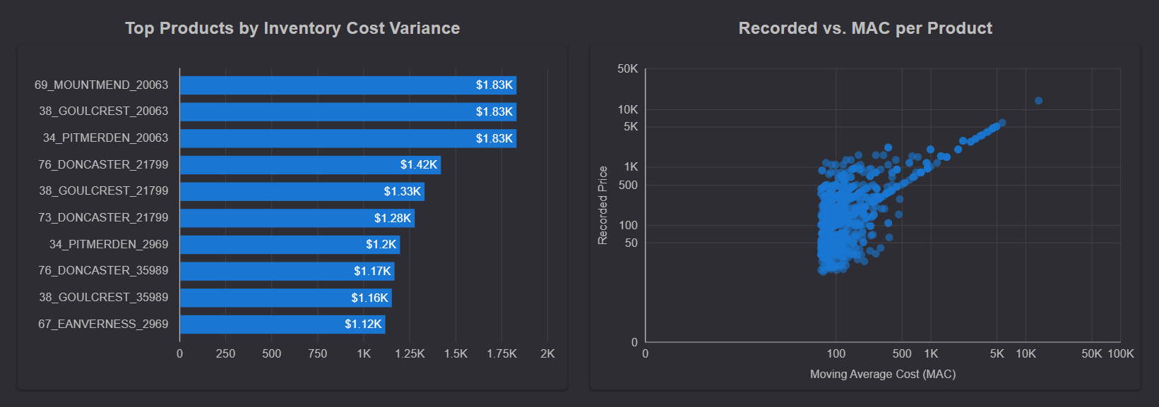
Beyond tracking inventory movement, understanding its true cost is essential for accurate financial reporting and pricing. This section applies the Moving Average Cost (MAC) method (which we discussed earlier in Section 2.4) to identify any cost differences.
- Inventory Cost Variance: The bar chart “Top Products by Inventory Cost Variance” helps us spot items with the biggest differences between their recorded cost and their calculated MAC. Products like 69_MOUNTMEND_20063 and 38_GOULCREST_20063 show notable differences (e.g., $1.83K). These differences mightindicate data issues or unexpected price changes that need investigation to ensure our inventory is valued correctly.
- Cost Alignment Check: The scatter plot “Recorded vs. MAC per Product” compares recorded costs to MAC for all products. Most products fall close to the diagonal line, meaning their costs align well. Any outliers on this chart signal inconsistencies that could impact profitability and require further review.
📝 Summary
This comprehensive dashboard provides an integrated view of Bibitor’s inventory dynamics. It highlights product sales velocity, slow-moving items, and key performance drivers by vendor and store. It also provides important insights into inventory cost accuracy. By visualizing movement trends, efficiency issues, and valuation gaps, the dashboard helps Bibitor optimize inventory, refine purchasing, ensure financial accuracy, and improve overall profitability.
📌 Final Takeaways
Through a combination of robust SQL analysis and interactive dashboards, this case study provided Bibitor with deep, actionable insights into its core operations. By translating complex data into clear visuals, we’ve provided a full understanding of:
- Vendor performance
- Inventory movement
- Product-level cost accuracy
Key insights, such as identifying top-performing and slow-moving products, evaluating vendor efficiency, and highlighting cost differences, help Bibitor make more informed decisions. Whether it’s improving stock turnover, refining purchasing strategies, or ensuring accurate financial reporting, the findings presented here offer a strong foundation for optimizing operations, increasing efficiency, and building lasting profit.
This data-driven approach not only reveals what’s happening — it also tells Bibitor what steps to take next.